2. Fitting Example (NLSF & MLE) in CPU - Bi-exponential FLI data processing

A simulated, full 3-D fluorescence lifetime image dataset of a two-well plate is generated (using the same simulator as the “Whole Image Simulation” example). Each well is assigned a different set of lifetime / FRET parameters. The data is then processed with fitted pixel by pixel with two estimators and the phasor method:

• Non-linear least squares (NLSF): minimizes the sum of squared residuals between the IRF-convolved model and the decay.

• Maximum likelihood estimation (MLE): maximizes the Poisson log-likelihood of the photon counts. It models the counting statistics directly, so it remains accurate at low photon counts, where least squares becomes biased.

This example walks through:

• Simulating the two-well FLI data and inspecting the ground-truth parameters

• Comparing NLSF and MLE on a single pixel

• Fitting the whole image with NLSF and with MLE

• Comparing the fitted maps and their distributions with the ground truth

• Inspecting the fit and residuals at individual pixels

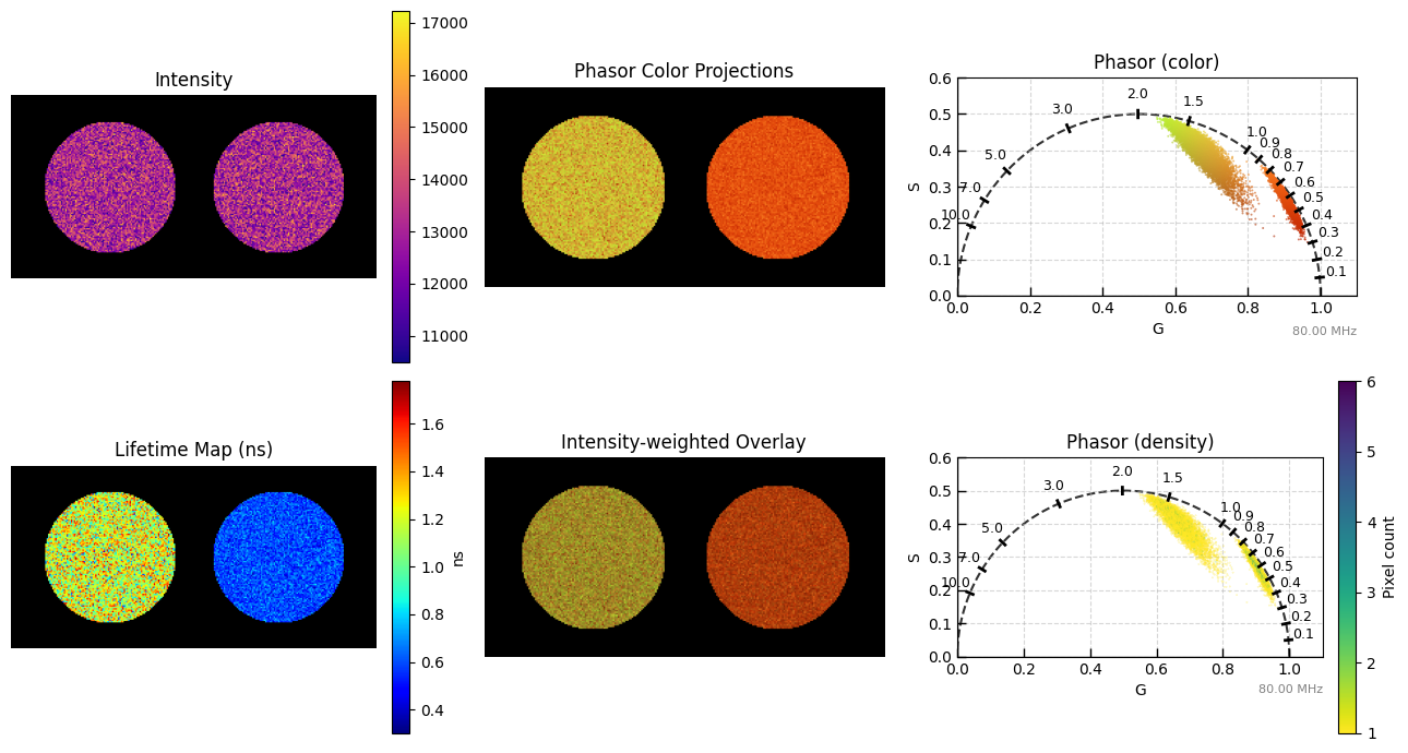
• The phasor computation, with pixel-wise IRF calibration to benchmark the results.

• Phasor plot and pixel-wise phasor color overlays

Author - Vikas

## importing the modules required for this work
import sys

import numpy as np

sys.path.insert(0, "ex_helper")  # local helper for synthetic image generation

from sim_general_image import ROIMaskGenerator

from pyfli.analysis.utils import random_true_pixel
from pyfli.analyticalWorkflow import AnalyticalHelpers
from pyfli.data_cc import Normalization
from pyfli.data_text import MessageDisplay
from pyfli.data_vnp import ColorProcessor, DataViewer
from pyfli.io import DataOperations
from pyfli.phasor.phasorS import PhasorAnalyzer
from pyfli.simulator import FLIModelImageGenerator

2.1. Loading the IRF

# Path to the local IRF file
IRF_PATH = "<select file/folder path>"

loader = DataOperations(irf_path=IRF_PATH)
irf_data = loader.load_irf()

gate_delay = 12.5 / irf_data.shape[2]
num_gates = irf_data.shape[2]
freq = AnalyticalHelpers(
    laser_period=12.5, gate_delay=gate_delay, num_gate=num_gates
).freq_computation()

INFO:pyfli:Initiating IRF load from: <select file/folder path>

2.2. Simulation configuration

MODEL_TYPE selects the decay model for both the simulation and the fits. get_config builds a per-well configuration by overriding BASE_CONFIG.

# select the type of decay model to simulate
MODEL_TYPE = "bi-exponential"
if MODEL_TYPE == "bi-exponential":
    mono_fraction = 0.0
elif MODEL_TYPE == "mono-exponential":
    mono_fraction = 1.0
else:
    mono_fraction = 0.4  # fraction of mono-exponential model in sampled data

# Your constant, default configuration
BASE_CONFIG = {
    # Modular Noise
    "jitter": False,  # offset artifact (due to jitter)
    "dcr_on": True,  # Dark Count Rate (thermal background)
    "poisson": False,  # Shot noise — Large detector only
    "qe_on": True,  # Quantum efficiency scaling
    "read_noise_on": False,  # Gaussian read noise — Large detector only
    # Sensor
    "sensor_type": "discrete",  # "continuous" | "discrete"
    "bit": 12,
    "dcr": 0.08,  # Mean dark counts per bin
    "laser_feq": freq[1],  # Laser repetition rate (MHz) → period = 12.5 ns
    "round_on": True,  # Round photon counts to integers — Macro_sim only
    "clip_on": True,  # Clip at bit-depth ceiling — Macro_sim: max_adc_val; TCSPC: max_bin_count
    # Fluorescence Physics (FLI / FRET)
    "tau2": (1, 1),  # τ₂ ~ TruncNormal(mu=1 ns, sigma=0.5 ns)
    "tau2_dist": "beta",  # if dist "beta" or "normal" (default)
    "tau2_beta_range": (2.5, 0.1),
    "efficiency": (1, 1),  # FRET efficiency E ~ Beta(2, 5)  → [0.1, 1.0]
    "A1_fraction": (1, 1),  # Amplitude fraction A₁ ~ Beta(2, 5) → [0.05, 0.95]
    "photo_count": (2, 5),  # Peak intensity ~ Beta(2, 5) × max_adc - large detectors
    "mono_fraction": mono_fraction,  # Fraction of pixels forced mono-exponential (0.0 = all bi-exp)
    "n_cycles": (1_500_000, 2_000_000),  # Accumulation cycles — for photon counter
}

def get_config(**kwargs):
    """Create a config by overriding defaults with specific test parameters."""
    config = BASE_CONFIG.copy()
    config.update(kwargs)
    return config

# Shared plotting / phasor configuration used by the two-well example below
colorset = "rainbow"
freq_hz = freq[1] * 1e6
jet_m_well = ColorProcessor().lowest_zero("jet")
bg_color = "black"  # either "black" or "white"
ph_cols_ = "viridis_r"

2.3. Two wells example

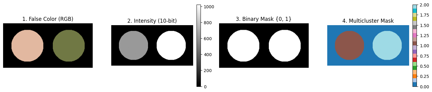
A two-well plate is simulated, with each well assigned a different set of ground-truth lifetime / FRET parameters.

from sim_general_image import WellPlateShape

h_well, w_well = 128, 256
generator_well = ROIMaskGenerator((h_well, w_well), top=10, bottom=10, left=10, right=10)
TwoWells = WellPlateShape(rows=1, cols=2, gap=0.15)

custom_intensities_well = [ 0.6, 1.0]
_ = generator_well.plot_preview(
    TwoWells,
    bit_depth=10,
    intensities=custom_intensities_well,
    show=True,
)

ROI0_well = {}
ROI1_well = get_config(
    tau2_beta_range=(0.1, 1.8),
    efficiency = (5, 2),  
    A1_fraction = (7, 13),
)
ROI2_well = get_config(
    tau2_beta_range=(0.2, 0.8),
    efficiency = (10, 10),  
    A1_fraction = (15, 10),
)

img_intensity_well = generator_well.generate_intensity_image(
    TwoWells, intensities=custom_intensities_well
)
img_cluster_well = generator_well.generate_cluster_mask(TwoWells)
b_bool_mask_well = generator_well.generate_binary_mask(TwoWells)

simulated_img_well = FLIModelImageGenerator(
    irf_data=irf_data[120, 40, :],
    intensity_image=img_intensity_well,
    roi_mask=img_cluster_well,
    roi_params=[ROI0_well, ROI1_well, ROI2_well],
    method="PHOTON_COUNTER",
    verbose=True,
    bool_mask=b_bool_mask_well,
)

gt_data_well = simulated_img_well.generate_image()

INFO:pyfli:Generating PHOTON_COUNTER FLI Image [128x256x256]...
Simulating Pixels:   0%|          | 0/32768 [00:00<?, ?px/s]

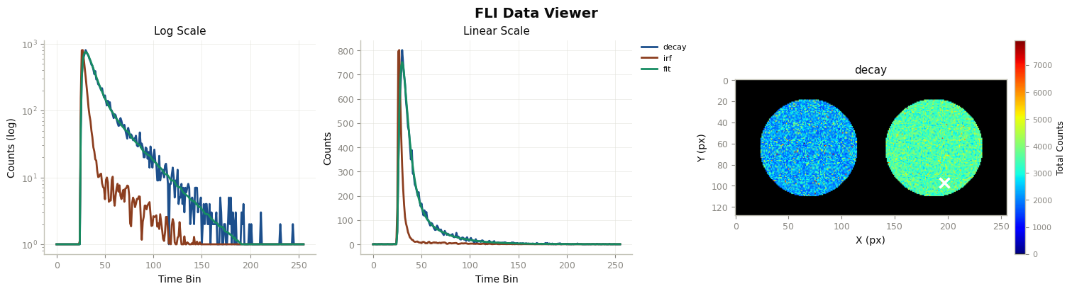
Check the decay, IRF, and fit at a randomly selected pixel.

_decay_well = gt_data_well["raw_data"]["decay"]
_irf_well = gt_data_well["raw_data"]["irf"]
x_well, y_well = random_true_pixel(b_bool_mask_well)
TRs_well = gt_data_well["results"]["TR_maps"]
maps_well = gt_data_well["results"]["maps"]
print(f"the non-zero pixel selected for probing is ({x_well}, {y_well})")
irf_norm_well = Normalization(_irf_well).norm_scale(_decay_well)
DataViewer().plot_fli_px(
    data_list=[_decay_well, irf_norm_well, TRs_well["fit_map"], TRs_well["residual_map"]],
    pixel=(x_well, y_well),
    mode=[0, 1, 2],
    mode2=[1],
    names=["decay", "irf", "fit"],
    cmap=jet_m_well,
)
_ = MessageDisplay().get_pixel_summary(data_maps=maps_well, px=(x_well, y_well))

the non-zero pixel selected for probing is (97, 197)

INFO:pyfli:
  Pixel (97, 197)
  ─────────────────────
  A         13877.4668
  α         0.5421
  τ₁        0.3039
  τ₂        0.9467
  R²        —
  Red.χ²    —
  Raw.χ²    —
  Pearson   —
  v-shift   0.0000
  h-shift   —
  ─────────────────────

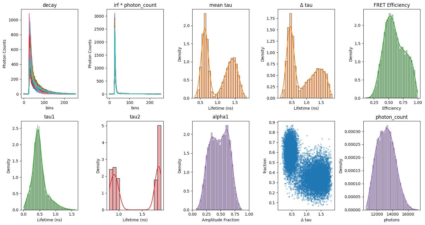
Distribution of the simulated ground-truth parameters across the image, before computing phasors.

import matplotlib.pyplot as plt
import seaborn as sns

res_well = gt_data_well["results"]["maps"]

b_bool_mask_well_bool = b_bool_mask_well.astype(bool)
valid_px_well = np.argwhere(b_bool_mask_well)
rng_well = np.random.default_rng(0)
sample_idx_well = rng_well.choice(len(valid_px_well), size=min(300, len(valid_px_well)), replace=False)
sample_px_well = valid_px_well[sample_idx_well]
decay_sample_well = _decay_well[sample_px_well[:, 0], sample_px_well[:, 1], :]
irf_sample_well = _irf_well[sample_px_well[:, 0], sample_px_well[:, 1], :]
photon_count_sample_well = res_well["photon_count_map"][sample_px_well[:, 0], sample_px_well[:, 1]]

tau1_valid_well = res_well["tau1_map"][b_bool_mask_well_bool]
tau2_valid_well = res_well["tau2_map"][b_bool_mask_well_bool]
alpha1_valid_well = res_well["alpha1_map"][b_bool_mask_well_bool]
tau_mean_valid_well = res_well["tau_mean_map"][b_bool_mask_well_bool]
efficiency_valid_well = res_well["fret_efficiency_map"][b_bool_mask_well_bool]
photon_count_valid_well = res_well["photon_count_map"][b_bool_mask_well_bool]
tau_dif_well = tau2_valid_well - tau1_valid_well

fig, axes = plt.subplots(2, 5, figsize=(15, 8))

axes[0, 0].plot(decay_sample_well.T)
axes[0, 0].set_title("decay")
axes[0, 0].set_xlabel("bins")
axes[0, 0].set_ylabel("Photon Counts")

axes[0, 1].plot((irf_sample_well * photon_count_sample_well[:, None]).T)
axes[0, 1].set_title("irf * photon_count")
axes[0, 1].set_xlabel("bins")
axes[0, 1].set_ylabel("Photon Counts")

sns.histplot(data=tau_mean_valid_well, ax=axes[0, 2], kde=True, stat="density", color="tab:orange", alpha=0.4)
axes[0, 2].set_title("mean tau")
axes[0, 2].set_xlabel("Lifetime (ns)")

sns.histplot(data=tau_dif_well, ax=axes[0, 3], kde=True, stat="density", color="tab:orange", alpha=0.4)
axes[0, 3].set_title("Δ tau")
axes[0, 3].set_xlabel("Lifetime (ns)")

sns.histplot(data=efficiency_valid_well, ax=axes[0, 4], kde=True, stat="density", color="tab:green", alpha=0.4)
axes[0, 4].set_title("FRET Efficiency")
axes[0, 4].set_xlabel("Efficiency")

sns.histplot(data=tau1_valid_well, ax=axes[1, 0], kde=True, stat="density", color="tab:green", alpha=0.4)
axes[1, 0].set_title("tau1")
axes[1, 0].set_xlabel("Lifetime (ns)")

sns.histplot(data=tau2_valid_well, ax=axes[1, 1], kde=True, stat="density", color="tab:red", alpha=0.4)
axes[1, 1].set_title("tau2")
axes[1, 1].set_xlabel("Lifetime (ns)")

sns.histplot(data=alpha1_valid_well, ax=axes[1, 2], kde=True, stat="density", color="tab:purple", alpha=0.4)
axes[1, 2].set_title("alpha1")
axes[1, 2].set_xlabel("Amplitude Fraction")
axes[1, 2].set_xlim(0.0, 1.0)

axes[1, 3].scatter(tau_dif_well, alpha1_valid_well, s=8, alpha=0.3)
axes[1, 3].set_xlabel("Δ tau")
axes[1, 3].set_ylabel("fraction")

sns.histplot(data=photon_count_valid_well, ax=axes[1, 4], kde=True, stat="density", color="tab:purple", alpha=0.4)
axes[1, 4].set_title("photon_count")
axes[1, 4].set_xlabel("photons")

plt.tight_layout()
plt.show()

2.4. Lifetime fitting: NLSF and MLE

For a bi-exponential model the fitted parameters are [S, alpha1, tau1, tau2, v_shift, h_shift]. Separating alpha1, tau1 and tau2 is harder than fitting a single lifetime, so the amplitude-weighted mean lifetime tau_mean is also compared below as the most robust summary of each pixel.

from pyfli.analysis.utils import plot_pixel_diagnostic
from pyfli.data_vnp import Plotter
from pyfli.solver import (
    BaseFLIFitter,
    BinnedFLIFitter,
    FittingComparator,
    FLICPUProcessor,
    MLEFLIFitter,
)

2.4.1. Single-pixel fit: NLSF vs MLE

Before fitting the whole image, FittingComparator fits one randomly selected pixel with both estimators and plots the fits side by side:

• "least_squares" uses BaseFLIFitter (NLSF)

• "poisson" uses MLEFLIFitter (Poisson MLE)

p0 (initial guess) and bounds are left as None, so the fitter derives its own initial guess from the data. Both can be passed in the parameter order given above.

p0 = None
bounds = None

xd_well, yd_well = random_true_pixel(b_bool_mask_well)
pixel_decay_well = _decay_well[xd_well, yd_well, :]
pixel_irf_well = _irf_well[xd_well, yd_well, :]

comparator = FittingComparator(freq, BaseFLIFitter, MLEFLIFitter)
comp_results_table, comp_fig = comparator.compare_selected(
    ["least_squares", "poisson"],
    y_data=pixel_decay_well,
    irf_data=pixel_irf_well,
    model_type=MODEL_TYPE,
    p0=p0,
    bounds=bounds,
    yscale="linear",
    plot=True,
)

┌──────────────────────────────────────────────────────────────┐
│  FLI Fitting Results  |  BI-EXPONENTIAL                      │
│  2 methods queued                                            │
└──────────────────────────────────────────────────────────────┘


┌────────────────┬──────┬─────────┬─────────┬──────────┬──────────┬─────────┬──────────┬──────────┬─────────┬──────────┐
│ Method         │ Type │       A │       α │       τ₁ │       τ₂ │      R² │   Red.χ² │   Raw.χ² │ v-shift │  h-shift │
├────────────────┼──────┼─────────┼─────────┼──────────┼──────────┼─────────┼──────────┼──────────┼─────────┼──────────┤
│ LEAST_SQUARES  │ NLSF │ 13731.14 │  0.5589 │    0.394 │    0.953 │  0.9961 │   1.1468 │   282.53 │    0.02 │   -0.000 │
│ POISSON        │ MLE  │ 13716.08 │  0.5424 │    0.388 │    0.933 │  0.9961 │   1.1061 │   280.04 │    0.10 │   -0.000 │
└────────────────┴──────┴─────────┴─────────┴──────────┴──────────┴─────────┴──────────┴──────────┴─────────┴──────────┘

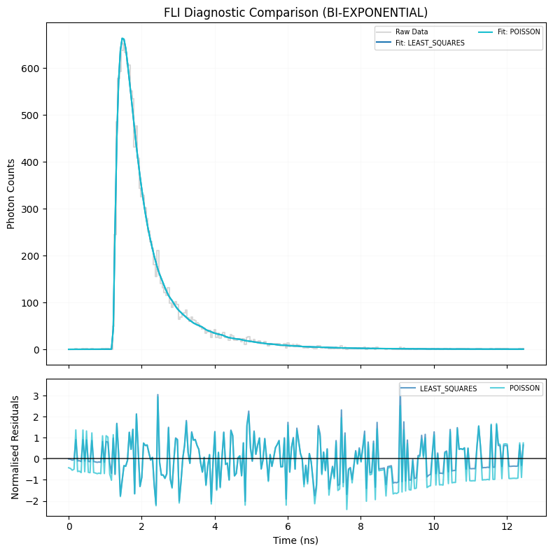
2.4.2. Whole-image fitting

Each pixel is fitted independently and in parallel on the CPU:

• FLICPUProcessor(freq, fitter_class) spreads the per-pixel fits over n_jobs worker processes. The fitter class sets the estimator family.

• BinnedFLIFitter(..., bin_radius=0) is the image-level entry point. A bin_radius of 0 fits every pixel as-is, and a larger radius sums each pixel with its neighbours first to raise the photon count.

• max_iter caps the optimizer’s function evaluations per pixel.

On a machine with a CUDA GPU, FLIGPUProcessor can be used in place of FLICPUProcessor to fit all pixels as one batch.

2.4.2.1. NLSF

MAX_ITER = 2000
N_JOBS = 7

nlsf_fitter = BinnedFLIFitter(FLICPUProcessor(freq, BaseFLIFitter), bin_radius=0)
results_nlsf = nlsf_fitter.fit(
    b_img=_decay_well,
    b_irf=_irf_well,
    estimator="least_squares",
    model_type=MODEL_TYPE,
    n_jobs=N_JOBS,
    data_name="simulated_wells_nlsf",
    max_iter=MAX_ITER,
)

INFO:pyfli:Engine: CPU Parallel Processor (via FLICPUProcessor)
Fitting Pixels (least_squares): 100%|██████████| 13226/13226 [01:28<00:00, 150.03px/s]

2.4.2.2. MLE

The same pipeline is run with MLEFLIFitter and the "poisson" estimator. MLE takes longer per pixel than NLSF.

MAX_ITER = 1500
mle_fitter = BinnedFLIFitter(FLICPUProcessor(freq, MLEFLIFitter), bin_radius=0)
results_mle = mle_fitter.fit(
    b_img=_decay_well,
    b_irf=_irf_well,
    estimator="poisson",
    model_type=MODEL_TYPE,
    n_jobs=N_JOBS,
    data_name="simulated_wells_mle",
    max_iter=MAX_ITER,
)

INFO:pyfli:Engine: CPU Parallel Processor (via FLICPUProcessor)
Fitting Pixels (poisson): 100%|██████████| 13226/13226 [04:30<00:00, 48.85px/s]

2.5. Comparing the results

Every fit result has the same layout: results["results"]["maps"] holds the parameter maps (alpha1_map, tau1_map, tau2_map, tau_mean_map, R2_map, reduced_chi2_map, …), and results["results"]["TR_maps"] holds the per-pixel fitted curves (fit_map) and residuals (residual_map).

2.5.1. Parameter maps

Rows: ground truth, NLSF, MLE. The lifetime color range is shared across rows and set from the ground truth.

experiments = {"NLSF": results_nlsf, "MLE": results_mle}
all_datasets = [res["results"]["maps"] for res in experiments.values()]
all_fitset = [res["results"]["TR_maps"] for res in experiments.values()]

keys_to_plot = ["tau1_map", "tau2_map", "tau_mean_map", "alpha1_map",]
sources = {"ground_truth": res_well, **dict(zip(experiments, all_datasets))}
tau_max = float(max(res_well["tau1_map"].max(), res_well["tau2_map"].max()))

_ = DataViewer().display_data(
    [maps[key] for maps in sources.values() for key in keys_to_plot],
    structure=(len(sources), len(keys_to_plot)),
    coord=None,
    data_names=[f"{key}_{name}" for name in sources for key in keys_to_plot],
    cmaps=[jet_m_well] * len(sources) * len(keys_to_plot),
    v_ranges=[(0, 1), (0, 2), (0, 2), (0, 1)] * len(sources),
    figsize=(20, 9),
    normalize=False,
    yscale="linear",
)

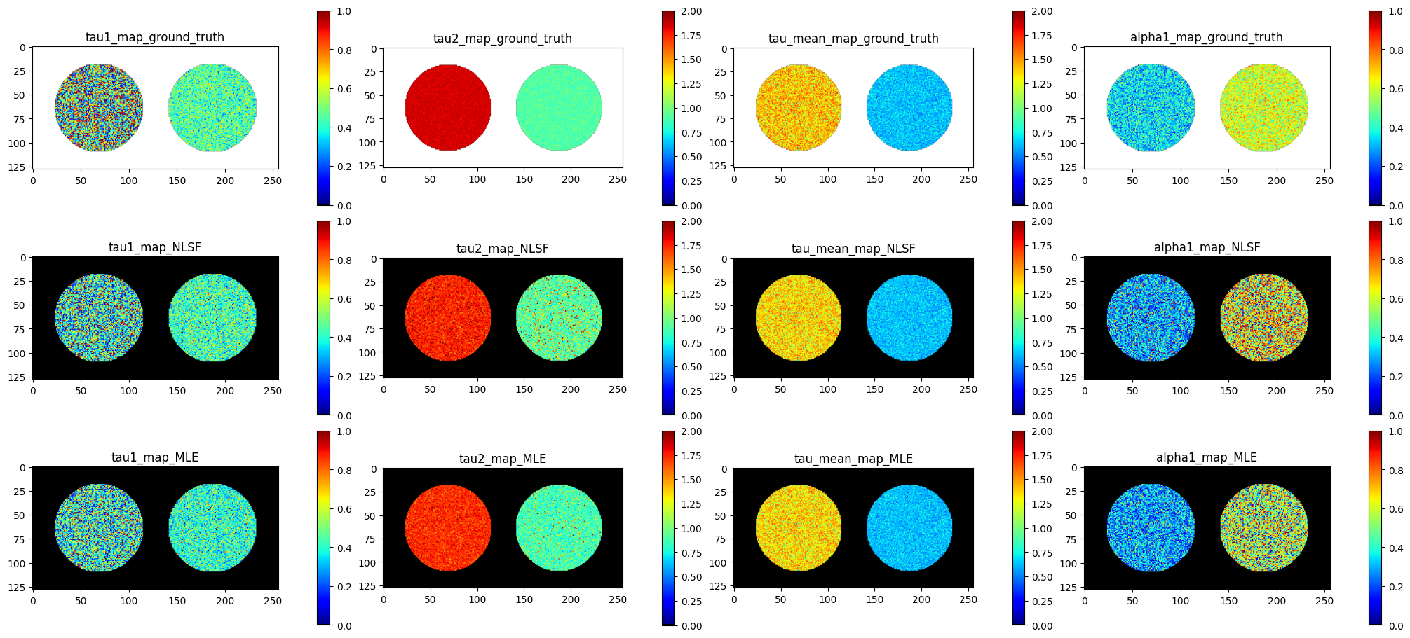
2.5.2. Parameter distributions

Plotter compares the parameter values of the well pixels across the sources. The operations dict is applied to every source: it keeps only pixels inside the mask, drops failed fits (NaN or zero) and discards values outside the threshold range. A list of dicts, one per source, can be passed instead to filter each source differently.

names = ["Ground truth"] + list(experiments)
plotter_ops = {
    "mask": b_bool_mask_well.ravel(),
    "remove_nan": True,
    "remove_zero": True,
    "threshold": (0, 7),
}

painter = Plotter(
    res_well,
    *all_datasets,
    values=keys_to_plot,
    style_config=["#AAB7B8", "#5DADE2", "#EC7063"],
    source_names=names,
    operations=plotter_ops,
)

fig = painter.make_plot(
    title="Bi-exponential parameters: ground truth vs NLSF vs MLE",
    graph_type="violin",
    point_type="strip",
    show_mean=True,
    show_median=True,
    show_significance=True,
    test_type="none",
    correction=False,
)

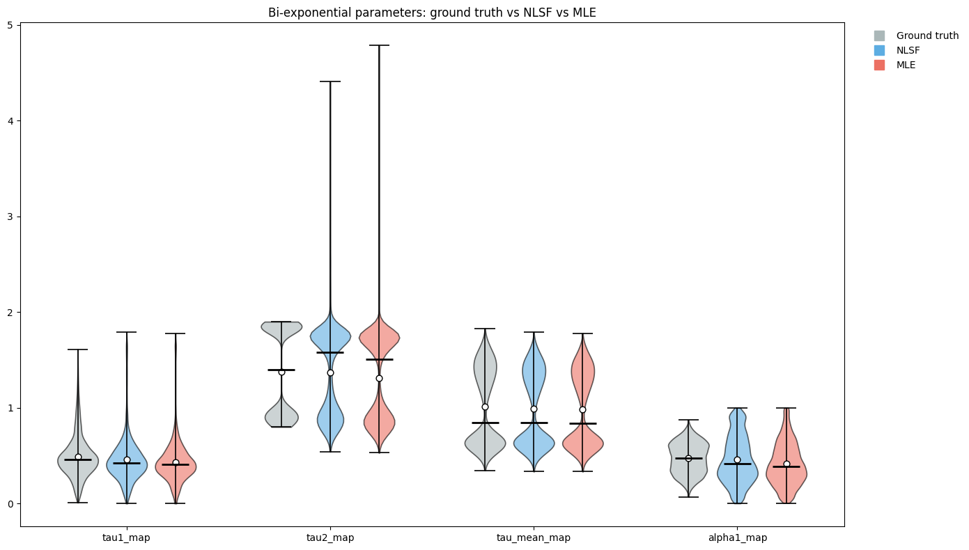
graph_type can also be "box", "swarm", "overlay", "raincloud" or "kde". Setting test_type to "paired" or "welch" adds significance tests between the sources.

2.5.3. Fits at a single pixel

plot_pixel_diagnostic overlays the NLSF and MLE fitted curves on the measured decay at one pixel, with the residuals below.

x_well, y_well = random_true_pixel(b_bool_mask_well)
_ = plot_pixel_diagnostic(
    _decay_well,
    all_fitset,
    list(experiments),
    mask=b_bool_mask_well,
    pixel=(x_well, y_well),
    t=None,
    yscale="log",
    raw_style="line",
    model_type=MODEL_TYPE,
)

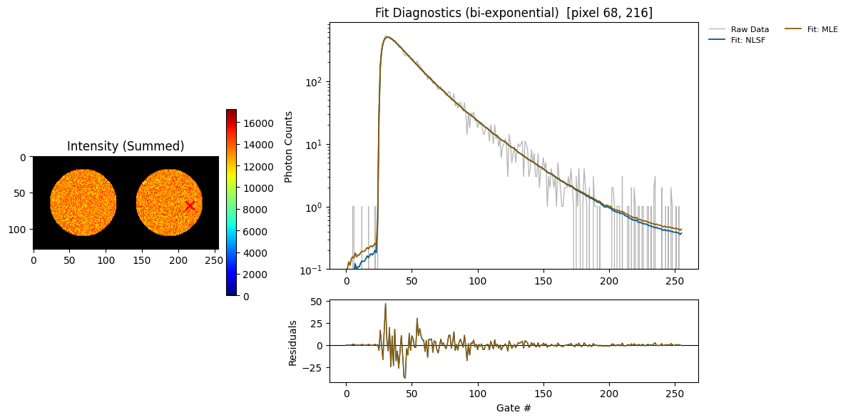
The same pixel is shown for each estimator, along with the fitted parameters and goodness-of-fit metrics (R², reduced χ²). The ground-truth values at this pixel are printed first for reference.

print(f"the non-zero pixel selected for probing is ({x_well}, {y_well})")
print("--- Ground truth ---")
_ = MessageDisplay().get_pixel_summary(data_maps=res_well, px=(x_well, y_well))
for name, maps, TRs in zip(experiments, all_datasets, all_fitset):
    print(f"--- {name} ---")
    DataViewer().plot_fli_px(
        data_list=[_decay_well, irf_norm_well, TRs["fit_map"], TRs["residual_map"]],
        pixel=(x_well, y_well),
        mode=[0, 1, 2],
        mode2=[0],
        names=["decay", "irf", "fit"],
    )
    _ = MessageDisplay().get_pixel_summary(data_maps=maps, px=(x_well, y_well))

INFO:pyfli:
  Pixel (68, 216)
  ─────────────────────
  A         13740.4316
  α         0.5310
  τ₁        0.7193
  τ₂        0.9768
  R²        —
  Red.χ²    —
  Raw.χ²    —
  Pearson   —
  v-shift   0.0000
  h-shift   —
  ─────────────────────

the non-zero pixel selected for probing is (68, 216)
--- Ground truth ---
--- NLSF ---

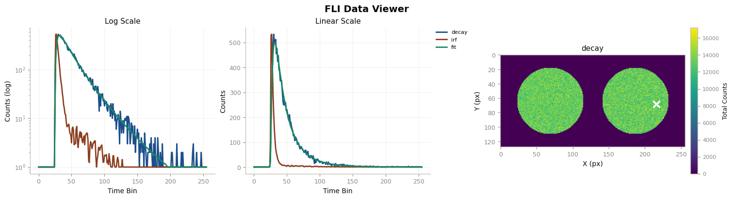
INFO:pyfli:
  Pixel (68, 216)
  ─────────────────────
  A         13860.1865
  α         0.0027
  τ₁        0.8360
  τ₂        0.8361
  R²        0.9958
  Red.χ²    1.0440
  Raw.χ²    258.7733
  Pearson   0.8221
  v-shift   0.0418
  h-shift   -0.0003
  ─────────────────────

--- MLE ---

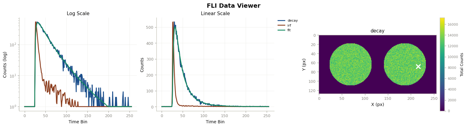
INFO:pyfli:
  Pixel (68, 216)
  ─────────────────────
  A         13850.7334
  α         1.0000
  τ₁        0.8351
  τ₂        0.8351
  R²        0.9959
  Red.χ²    1.0196
  Raw.χ²    257.5890
  Pearson   0.8179
  v-shift   0.1008
  h-shift   -0.0004
  ─────────────────────

2.6. Phasor computation and visualization

time_axis_ns_well = np.linspace(0, gate_delay * num_gates, _irf_well.shape[2])
phasor_well = PhasorAnalyzer(
    frequency_hz=freq_hz, time_axis_ns=time_axis_ns_well, n_harmonics=3
)
G_well, S_well = phasor_well.create_phasor_gpu(_decay_well)
Gc_well, Sc_well = phasor_well.calibrate_pixelwise(G_well, S_well, _irf_well)
tau_map_ns_well = phasor_well.compute_lifetime(Gc_well[0], Sc_well[0])

im2_well = phasor_well.plot_overlay_subplots(
    _decay_well,
    Gc_well[0],
    Sc_well[0],
    mask=b_bool_mask_well,
    colormaps=["plasma", "jet", "turbo_r", ph_cols_],
    figsize=(13, 7),
    xlim=(0, 1.1),
    bg_color=bg_color,
    transpose=False,
    kdeplot=False,
)